The example datasets
Load example, at the top right of the upload form, fills the form with a ready-made dataset and locks the panels; you then press Run PaintOmics as you would for your own data. It is the fastest way to see any part of PaintOmics work, and it is also how you check that a server is correctly installed.
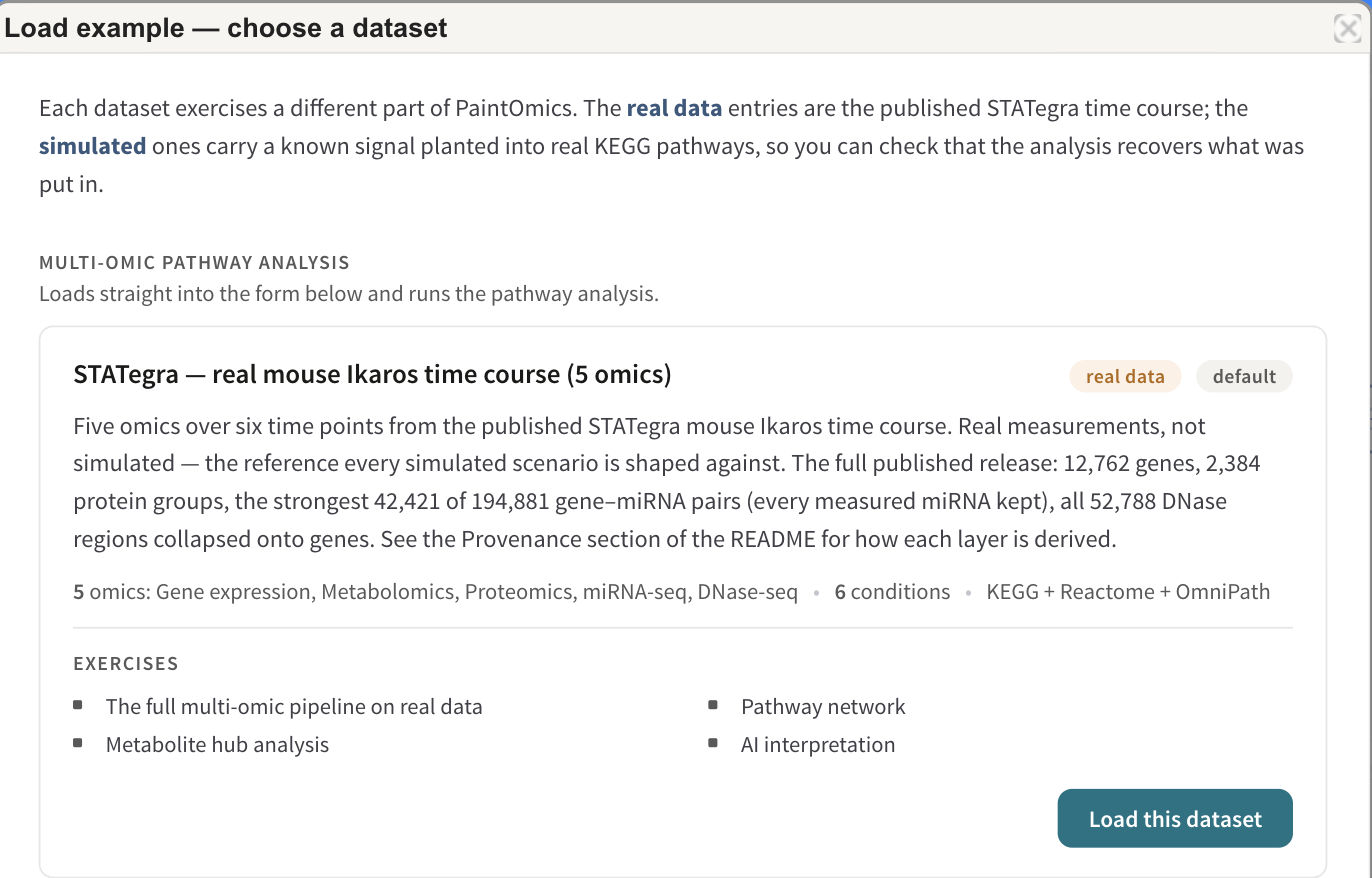
The dataset chooser. Each card names the omics, the number of conditions and the pathway databases the dataset was authored against, and lists what it is there to exercise. Load this dataset puts it on the form. The databases the job actually runs are the ones this server has installed for the organism, which can be more than the card lists.
Two kinds of dataset are offered, and the difference matters when you are judging a result.
Real data is the published STATegra mouse Ikaros time course — real measurements, with all the noise and all the unmatched identifiers of a real submission. Use these to see what your own data will look like.
Simulated datasets carry a known signal planted into real KEGG pathways. Nothing about the identifiers or the pathway structure is fake; only the values are constructed, so you can check that the analysis recovers what was put in. Because their features are drawn from KEGG's own gene universe, KEGG coverage on a simulated dataset is close to 100% by construction — which makes them the wrong datasets for comparing one pathway database against another. Use the STATegra ones for that.
Multi-omic pathway analysis
These load straight into the upload form and go to the pathway analysis when you press Run PaintOmics.
| Dataset | Data | What it is for |
|---|---|---|
| Gene expression — single condition | 1 omic, 1 condition, simulated | The smallest input PaintOmics accepts: one values file and one relevant-features list. The fastest way to see a pathway light up. |
| Gene expression — six conditions | 1 omic, 6 conditions, simulated | The ordinary shape of a time-course submission — one relevance list shared by every condition. Exercises the multi-condition heatmaps and per-condition colouring. |
| Gene expression — per-condition relevance | 1 omic, 6 conditions, simulated | The same time course, but with a relevant-features file holding one column per condition, so significance is tracked separately at each time point. |
| Multi-omic integration — five omics | 5 omics, 6 conditions, simulated | Transcriptomics, proteomics, transcription factors, metabolomics and miRNA over the same time points, sharing one planted signal so the layers agree. Exercises compound matching, the hub analysis and the pathway network. |
| STATegra — real mouse Ikaros time course | 5 omics, 6 conditions, real | The default. 12,762 genes, 2,384 protein groups, 42,421 gene–miRNA pairs and 52,788 DNase regions collapsed onto genes. This is the dataset every screenshot in this guide was taken from. |
| STATegra metabolomics — replicates and experimental design | 1 omic, 12 groups, real | The STATegra metabolomics with its 36 individual samples and an experimental design file instead of six averaged ratios. This is the dataset that turns the metabolite class activity test into a permutation test on your own replicates. |
Datasets that need a pre-processing step
These load one panel into the same upload form. Pressing Run PaintOmics runs that panel's pre-processing step first, and its output then feeds the ordinary pathway analysis.
| Dataset | Step it loads | What it is for |
|---|---|---|
| Regulatory omics — miRNA to genes | Regulatory omics — pairwise | miRNA quantification plus a target-prediction table; the step pairs each miRNA with its targets and hands GENE:::miRNA rows on to the pathway analysis. |
| Region-based omic — DNase-like regions | Region-based omics | BED-like regions with a matching synthetic GTF, so region-to-gene assignment runs on a fresh checkout that has no full mouse annotation. Signal regions sit in promoters; 200 intergenic decoys do not. |
| Regulatory omics — MORE joint model | MORE | Per-sample expression with three replicates per group, an experimental design matrix, and two candidate regulatory omics with association files. Each target is a noisy linear function of one known regulator, so what MORE should find is written down. |
| STATegra — DNase regions (real) | Region-based omics | All 52,788 consensus DNase-seq regions, unmapped. Needs the full mouse annotation, which a deploy step fetches and a fresh checkout does not have. |
| STATegra — miRNA to genes (real) | Regulatory omics — pairwise | The unmapped STATegra miRNA quantification with the full miRBase-to-Ensembl target table. |
| STATegra — real expression against a real TF network | MORE | GSE75417 against the literature-curated half of the TFLink v1.0 mouse network: 957 genes, 387 transcription factors, 36 samples, 12 groups, nothing subsampled. Real measurements and no planted signal. |
The same two steps are also available on their own, without a pathway analysis, under Tools ▸ From Regions to Genes and Tools ▸ From miRNA to Genes.
Getting the files
Download example data on the upload form — listed as PaintOmics example
data under More ▸ Resources — gives you the whole catalogue as files you
can open and copy. It is built from
the catalogue of the server you are using, so it always matches what Load
example offers, and it includes a HOW-THIS-DATA-WAS-MADE.md explaining
which datasets are simulated and exactly how each one was generated.
An example job is read-only
When a dataset is loaded, the omic panels are fixed: the organism, databases and files come from the server's catalogue and cannot be edited. Reset returns you to an empty upload form, and Load another example switches dataset.