Comparing three or more groups
PaintOmics compares any number of groups. Give it one log2 fold-change column per contrast, and a relevant-features file with one list of significant features per contrast; every pathway then gets its own p-value for each comparison, beside one that combines them.
This page runs the whole workflow on a three-group example — mouse RNA-seq and
lipidomics, groups Ctrl, TrtA and TrtB, four animals each — from raw
counts to the painted pathways. The red numbers on the screenshots are the
numbered steps in the text.
What you need
- The example data:
paintomics-three-group-example.zip
(0.6 MB). It holds raw RNA-seq counts and lipid intensities for the 12
animals, an R script that turns them into PaintOmics files, the four files the
script makes, and the answer key
PLANTED_SIGNAL.tsv. If you only want to try PaintOmics, the four upload files are already in itspaintomics_inputsfolder: skip to Step 2. - R 4.2 or later with DESeq2 and limma, for Step 1 only. The script was tested with R 4.6.0 and DESeq2 1.52.0.
- paintomics.org, or your own installation with Mus musculus.
The example data are simulated
The gene and compound identifiers and the pathway structure are real mouse KEGG; the numbers are not. Seven KEGG pathways were made to change — some in both treatments, some in one — so you can check that the analysis recovers what was put in. Draw no biological conclusion from them.
Step 1 — Make one column per contrast
PaintOmics paints one value per feature per column, so three groups become
pairwise contrasts. Unzip the example and run Rscript make_paintomics_inputs.R
in that folder; it writes four files to paintomics_inputs/ in under a minute.
The only part you edit is the settings block at the top of the script:
reference_group <- "Ctrl"
group_levels    <- c("Ctrl", "TrtA", "TrtB")

# one entry per column PaintOmics will show: name = c(numerator, denominator)
contrasts <- list(
  TrtA_vs_Ctrl = c("TrtA", "Ctrl"),
  TrtB_vs_Ctrl = c("TrtB", "Ctrl"),
  TrtB_vs_TrtA = c("TrtB", "TrtA")
)
fdr_cutoff <- 0.05   # adjusted p-value that makes a feature "relevant"
What the script does with it:
- RNA-seq, with DESeq2. It strips the Ensembl version suffix
(
ENSMUSG00000000001.5becomesENSMUSG00000000001, because gene identifiers are matched exactly), drops genes with fewer than 10 reads in 4 samples, fits~ grouponce, and takesresults(dds, contrast = c("group", "TrtA", "Ctrl"))for each contrast. - Lipids, with limma. It keeps species detected in at least 75% of the
samples of one group, fills the remaining gaps with half that species'
smallest value, sums the species into their KEGG lipid class — every PC
species into
C00157, Phosphatidylcholine — takes log2 and tests each contrast. - It writes the log2 fold changes as the values files, and the features with FDR < 0.05 in each contrast as the relevant-features files.
| File | Header row | Then |
|---|---|---|
rnaseq_values.tsv |
#gene_id TrtA_vs_Ctrl TrtB_vs_Ctrl TrtB_vs_TrtA |
one gene per row, one log2 fold change per contrast |
rnaseq_relevant.tsv |
TrtA_vs_Ctrl TrtB_vs_Ctrl TrtB_vs_TrtA |
one list of significant genes per column — 230, 315 and 398 here — with blank cells where a list ends |
lipids_values.tsv |
#kegg_id TrtA_vs_Ctrl TrtB_vs_Ctrl TrtB_vs_TrtA |
one KEGG compound per row |
lipids_relevant.tsv |
TrtA_vs_Ctrl TrtB_vs_Ctrl TrtB_vs_TrtA |
one list per column — 10, 9 and 11 compounds |
Two rules make this work. The values header starts with # and the
relevant-features header does not: with two contrasts, a # there makes
PaintOmics read the file as a regulator–target pair list (see
per-condition relevance).
And the contrast names must be the same, in the same order, in all four files —
every omic in a job has to carry the same number of value columns.
Step 2 — Choose the organism and describe the design
Open PaintOmics and scroll to 1. Organism selection.
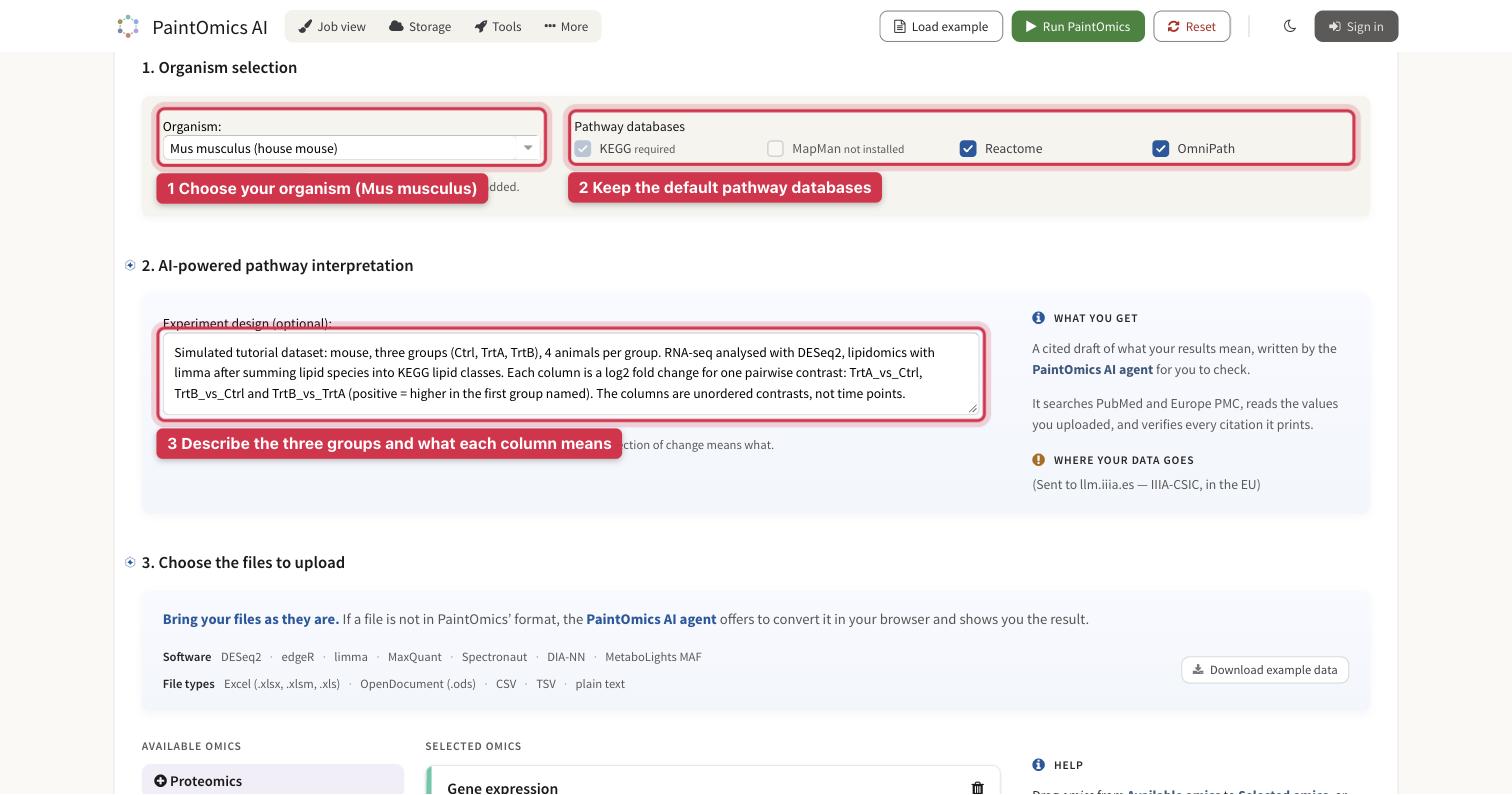
The upload form, with the three things set in this step.
1. Organism: type Mus musculus and pick Mus musculus (house mouse).
2. Pathway databases: leave the defaults. For mouse these are KEGG, Reactome and OmniPath.
3. Experiment design: say what the groups are and what each column means. The AI interpretation reads this text together with your column headers, and it needs to know that the columns are pairwise contrasts rather than time points. The example used:
Mouse, three groups (Ctrl, TrtA, TrtB), 4 animals per group. RNA-seq analysed with DESeq2, lipidomics with limma after summing lipid species into KEGG lipid classes. Each column is a log2 fold change for one pairwise contrast: TrtA_vs_Ctrl, TrtB_vs_Ctrl and TrtB_vs_TrtA (positive = higher in the first group named). The columns are unordered contrasts, not time points.
Step 3 — Upload the four files and run
Scroll to 3. Choose the files to upload. The Gene expression and Metabolomics cards are already on the form; the lipids go in the Metabolomics card.
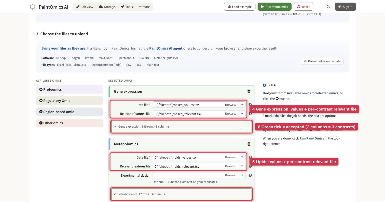
Both cards green: each file was read with three value columns.
4. Gene expression: in Data file choose rnaseq_values.tsv, and in
Relevant features file choose rnaseq_relevant.tsv.
5. Metabolomics: the same with lipids_values.tsv and
lipids_relevant.tsv. Leave Experimental design empty; it is for files
with one column per sample.
6. Wait for the green tick. The browser checks each file as you pick it, and
3 columns means it read your three contrasts. Amber offers a one-click
repair; red means the file is in the wrong shape — see
what happens when you pick a file.
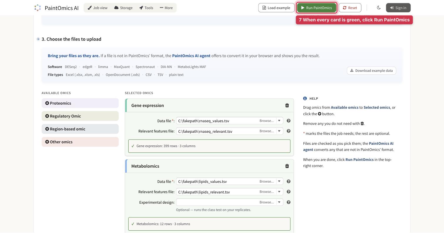
7. When both cards are green, click Run PaintOmics in the top-right corner. The job uploads, queues and maps your identifiers; for the example this took under a minute.
Step 4 — Check the identifier mapping
The second screen reports how many of your features PaintOmics could place on pathways. In the example, all 15,094 genes and all 33 lipid compounds map to KEGG.
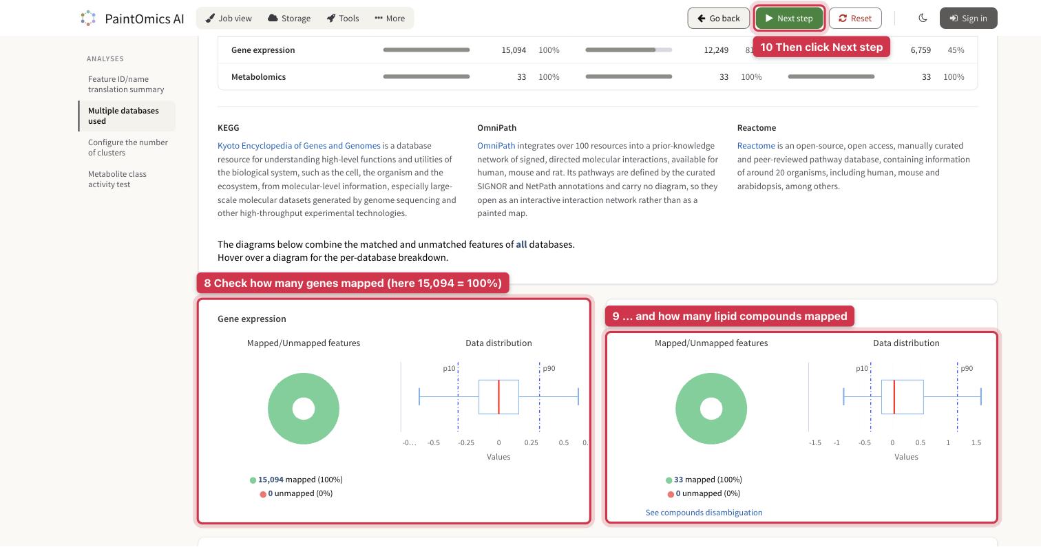
8. Gene expression card: green is mapped, red is not. With real data, aim for most of the file to be green; when a file matches poorly lists what to try.
9. Metabolomics card: the same for the lipids. If few of them map, they are probably species-level identifiers — see the last section.
10. Further down, the Metabolite class activity test shows a threshold of 0.05. That is the FDR cut-off the script used, so leave it. Click Next step in the top bar; the pathway analysis takes about a minute.
Step 5 — Read one p-value per contrast
On the results page, click Pathway enrichment in the left menu.
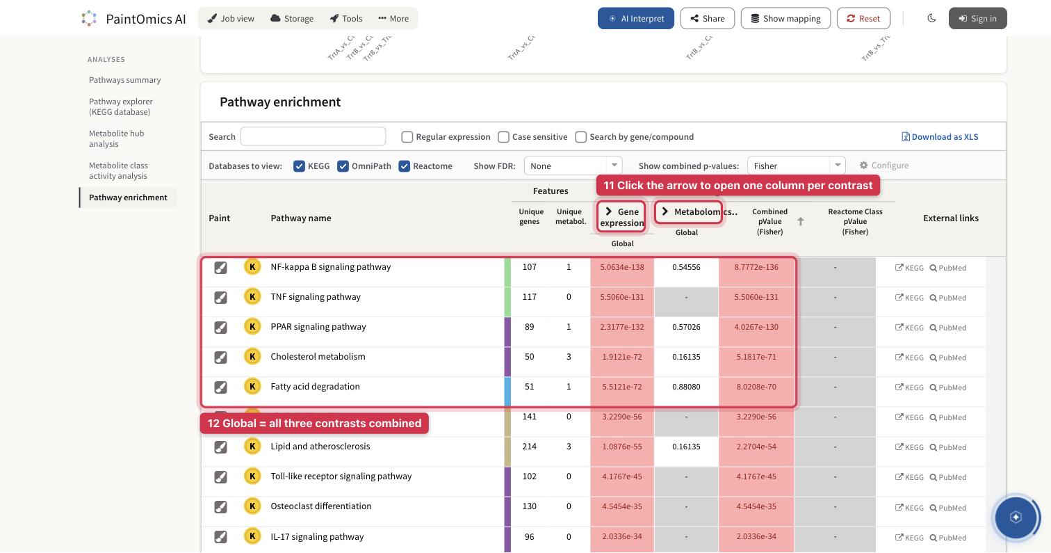
11. Each omic's column header carries an arrow, because your relevant-features files hold one list per contrast. Click the arrow next to Gene expression.
12. Until you do, the column shows only Global: the three contrasts combined by Fisher's method. It ranks the pathways, but it does not say which group drives them.
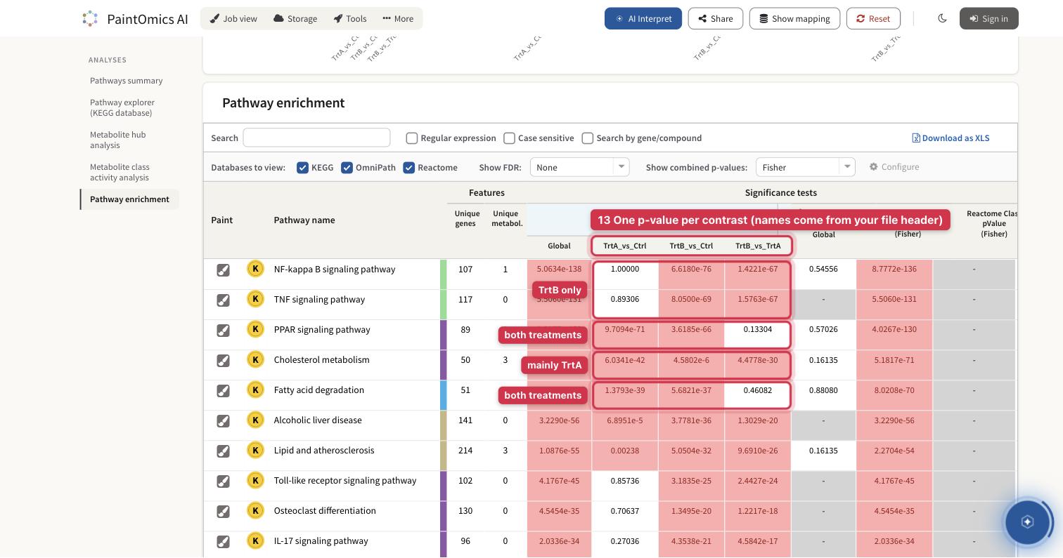
13. The column opens into Global plus one sub-column per contrast, named from your file's header. Each cell is a separate enrichment test against that contrast's own significant genes; cells at or below 0.065 are tinted red, more deeply the smaller they are.
Read each row across the three contrast columns:
| Pattern | TrtA_vs_Ctrl | TrtB_vs_Ctrl | TrtB_vs_TrtA | In the example |
|---|---|---|---|---|
| Changed by both treatments alike | small | small | not significant | PPAR signaling: 9.7e-71 · 3.6e-66 · 0.13; Fatty acid degradation: 1.4e-39 · 5.7e-37 · 0.46 |
| Changed by TrtA only | small | not significant | small | Steroid biosynthesis: 1.1e-14 · 0.41 · 2.2e-12 |
| Changed by TrtB only | not significant | small | small | NF-kappa B signaling: 1.00 · 6.6e-76 · 1.4e-67; TNF signaling: 0.89 · 8.1e-69 · 1.6e-67 |
The third contrast is what separates "both" from "one": a response the two
treatments share cancels out in TrtB_vs_TrtA. Overlapping pathways can blur
the pattern. Cholesterol metabolism (6.0e-42 · 4.6e-6 · 4.5e-30) was changed in
TrtA only, yet reaches 4.6e-6 in TrtB, because 9 of its 50 genes also belong to
the PPAR pathway, which responds in both groups. Check the genes (Step 7) before
calling a pathway specific to one group.
The Combined pValue column merges each omic's Global value across omics: use it to rank, and the contrast columns to explain. Download as XLS exports only the visible columns, so open the contrasts before exporting.
Step 6 — The lipids, per contrast
Click the arrow next to Metabolomics to open its contrasts as well; close the Gene expression group first if the table runs off the screen.
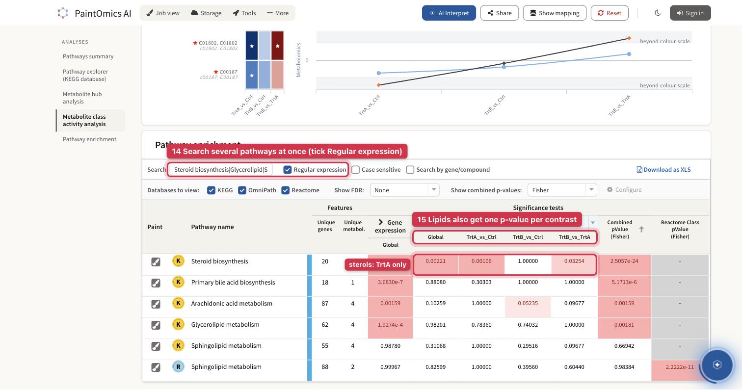
14. To look at several pathways at once, tick Regular expression and search
Steroid biosynthesis|Glycerolipid|Sphingolipid metabolism|Arachidonic|Primary bile.
15. The lipids get one p-value per contrast too. Steroid biosynthesis reads
0.0011 in TrtA_vs_Ctrl and 1.00 in TrtB_vs_Ctrl: the sterols fall in
TrtA only, as the genes did.
Expect lipid p-values to be weaker than gene p-values. Summed to KEGG classes, a lipid panel gives each pathway between one and five measured compounds, so even a real change rarely reaches a small p-value — arachidonic acid metabolism in TrtB reads 0.052. Read the lipids on the painted pathway instead (next step). The metabolite hub analysis on the same page helps too: in the example its top hits are planted compounds — leukotriene B4, triacylglycerol, cholesterol ester and cholesterol.
Step 7 — Paint a pathway and read its heatmap
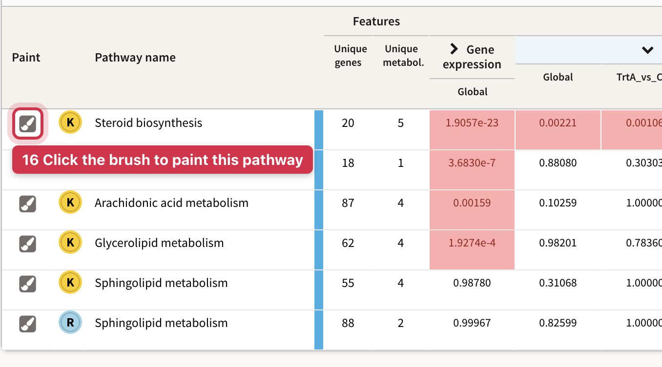
16. Click the brush in a row's first column. Steroid biosynthesis is a good first choice in the example, because it carries both genes and lipids.
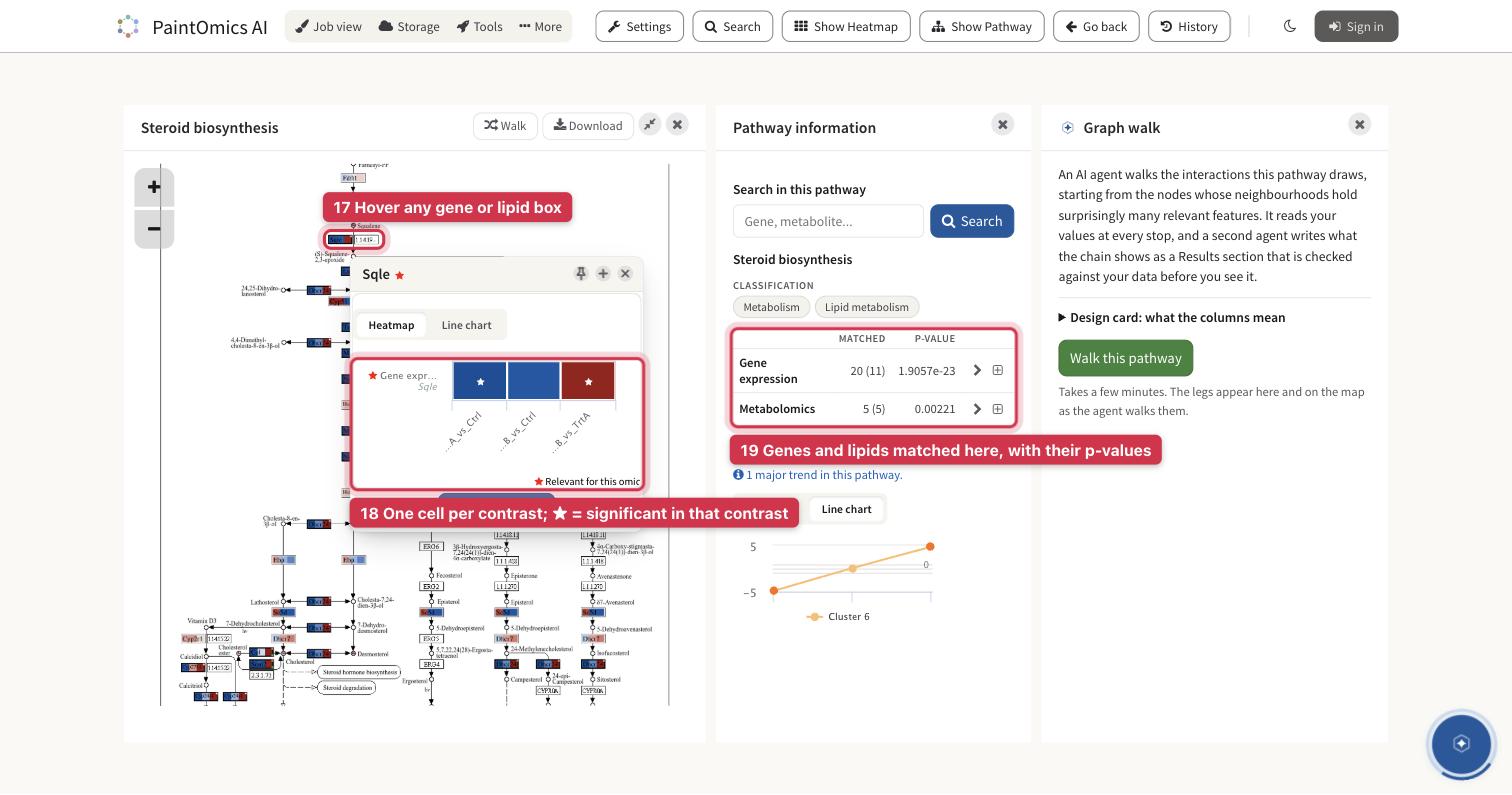
17. Every painted gene and compound box holds one cell per contrast, left to right in your column order. Hover a box to see its values.
18. The pop-up has one cell per contrast, and a star marks the contrasts in
which that feature is on your relevant list. Sqle is starred in
TrtA_vs_Ctrl (log2 fold change −1.36) and in TrtB_vs_TrtA (+0.91), and
not in TrtB_vs_Ctrl (−0.46).
19. Pathway information gives the pathway's matched features and p-values: 20 genes, 11 of them relevant, and 5 lipids, all relevant.
The colours saturate early. By default the scale runs between the 10th and 90th percentiles of your data — ±0.31 log2 for these genes — so −0.46 is already full blue. Trust the stars for significance, and widen the range under Settings → Coloring options → Reference values if you want to; see where the ends of the scale come from.
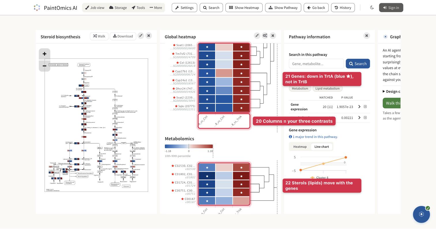
20. Click Show Heatmap in the top bar, then Apply. Each omic gets a block whose columns are your three contrasts; Heatmaps covers the options. Download, in the panel's header, saves the whole heatmap — every omic and every row, with the contrast names in full — as a PNG for a report or an SVG to edit.
21. The relevant genes of Steroid biosynthesis are blue and starred in
TrtA_vs_Ctrl, near zero in TrtB_vs_Ctrl, and red in TrtB_vs_TrtA:
lower in TrtA than in either other group.
22. The five sterols — cholesterol ester, desmosterol, lanosterol, squalene and cholesterol — follow the genes. Agreement between genes and lipids, contrast by contrast, is the multi-omic evidence for an effect specific to one group.
Step 8 (optional) — The AI interpretation
On a server that offers it — paintomics.org does — the AI interpretation runs in the background while you browse the results. When the round mark in the bottom-right corner shows a green tick, click it, or AI Interpret in the results toolbar.
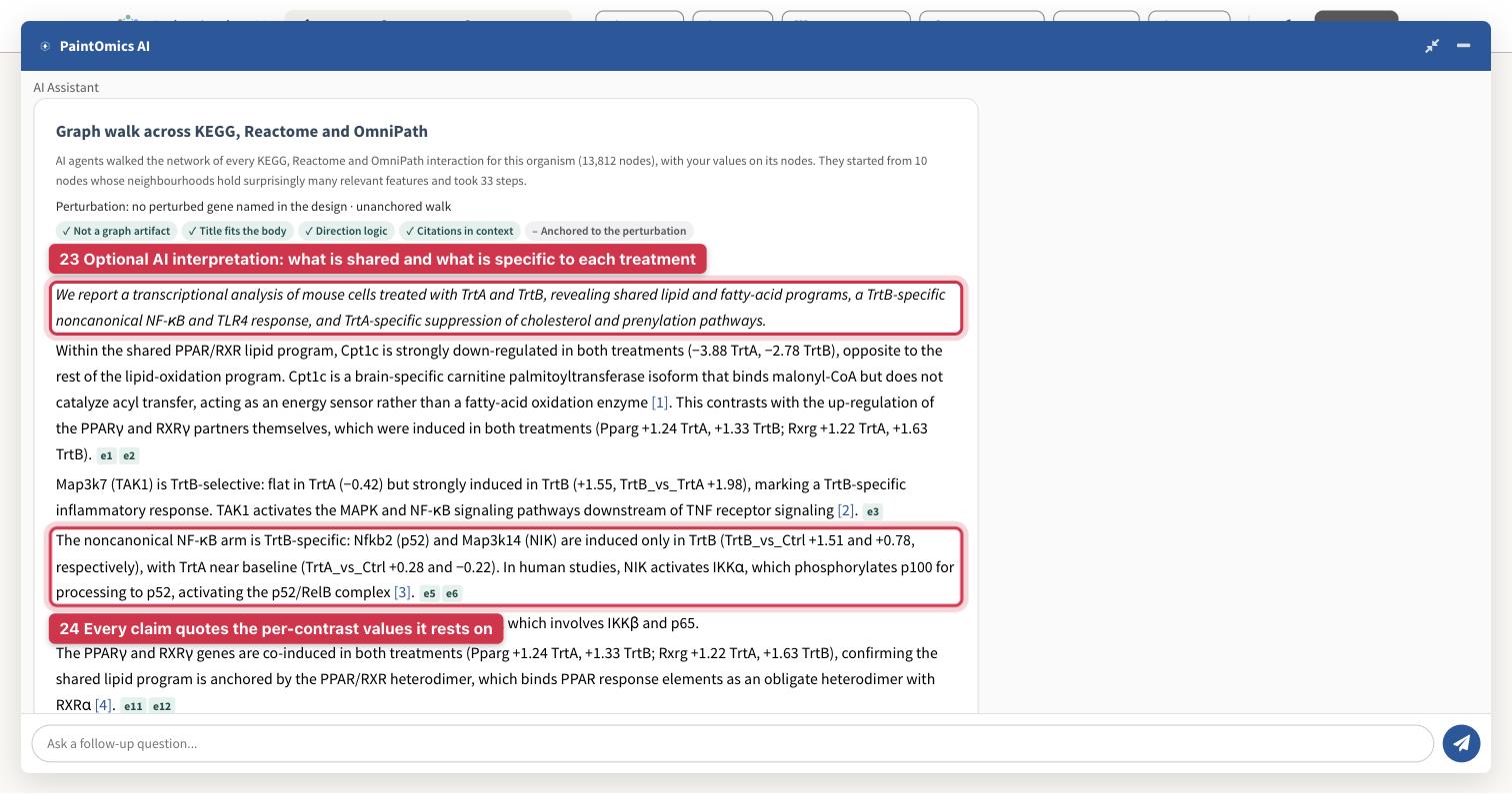
23. Because the design text named the contrasts, the summary sorts the result the way the signal was planted: shared lipid and fatty-acid programmes, a TrtB-specific NF-κB response, and TrtA-specific suppression of the cholesterol and prenylation pathways.
24. Every claim quotes the per-contrast values it rests on, and every citation is checked against the paper.
Treat it as a first draft to check against your own reading of Steps 5 to 7. On this simulated example, its literature statements describe real genes, not findings about TrtA or TrtB. See The interpretation.
On your own data
Replace the four files in raw_data/ with yours, keeping their layout, and edit
the settings block:
- Groups and contrasts. Put your group names in
group_levelsand keep the contrasts you need. Two contrasts against a control are fine; the script still writes the header row that a two-column relevant-features file needs. - Gene identifiers. The first column of the counts table is the gene
identifier. Ensembl, NCBI Gene and gene symbols all map for mouse; symbols are
case-sensitive (
Gnai3, notGNAI3). See supported identifiers. - Lipids. List each of your lipid classes in
lipid_class_to_kegg.tsv, with the KEGG compound it is drawn as. KEGG draws lipids per class, so a species-level ChEBI or SwissLipids identifier has no KEGG entry to map to. - No natural reference group — three tissues, say? Use the group means
instead: as values, each group's mean log2 expression minus the mean of the
three; as the one relevant list, the genes significant in
DESeq(dds, test = "LRT", reduced = ~ 1). You then get one test per pathway, without the split by contrast.
| Symptom | Cause | Fix |
|---|---|---|
| No arrow on the omic column, so no per-contrast p-values | The relevant-features file is a single list | One column per contrast, under a plain header of contrast names |
| An omic is refused for its number of columns | Every omic in a job must carry the same number of value columns | The same contrasts, in the same order, in the RNA-seq and the lipid files |
| Huge values such as 2017143390864550, or the file turns red | A decimal comma was lost: 2,0171… written by a spreadsheet set to a comma locale |
Write the files from R and do not re-save them in a spreadsheet. On a tab-separated file, the amber Use dots as the decimal mark repair fixes it |
| Few genes map | Ensembl version suffixes such as .5, or the wrong organism |
The script strips suffixes; check the organism in Step 2 |
| Almost no lipids map | Species-level identifiers (PC 34:1, or the ChEBI number of one species) |
Sum species into classes and use the class's KEGG compound (C00157 PC, C00422 TG). A ChEBI identifier maps only when ChEBI cross-references it to KEGG |
| A two-column relevant-features file behaves oddly | With no header, or a header starting with #, two columns of identifiers are read as a regulator–target pair list |
A plain header row of contrast names, without # |
| The contrasts show up as Condition 1, 2, 3 instead of their names | A contrast name with four or more digits in a row, or a colon (Day1000, KO:WT), makes the header look like data, so it is read as a row of identifiers |
Short names such as TrtA_vs_Ctrl |
The DESeq2 contrast syntax the script uses is the one described in the DESeq2 vignette.